Path simplification
To simplify the neural network’s task of representation learning, it can make sense to simplify paths.
Generally, the aim is to reduce the number of points that form a shape. But, in some implementations and for some input examples, the number of points can increase if the resolution of a curve would otherwise be too low.
Simplification approach
(1) Split path at corner points to preserve their location
If the SVG input only consisted of smooth curves, the simplification step could simply be to reparametrize points on that curve so that they are placed equidistantly from one another. However, since SVG shapes contain sharp angles and, thus, corners, these points should not be changed.
Consequently, paths are first split at points that form a sharp angle. This is measured by the angle between the incoming and the outcoming tangent. If the angle is smaller than some threshold (e.g. DeepSVG uses a threshold of \(\eta = 150°\)), then the angle is considered sharp.
(2) Polyline simplification: Ramer-Douglas-Peucker algorithm
For line segments, the Ramer-Douglas-Peucker algorithm can be applied which was introduced in “Algorithms for the Reduction of the Number of Points Required to Represent a Digitized Line or its Caricature” (1973). The algorithm is also known as just Douglas-Peucker algorithm. Urs Ramer developed the solution independently and published it in “An iterative procedure for the polygonal approximation of plane curves” in 1972.
This simplification algorithm was used in Ha and Eck (2017) and Carlier et al. (2020). Ha and Eck note:
For most single-class datasets, sketch-rnn is capable of modelling sketches up to around 300 data points. The model becomes increasingly difficult to train beyond this length. For our dataset, we applied the Ramer–Douglas–Peucker algorithm to simplify the strokes of the sketch data to less than 200 data points while still keeping most of the important visual information of each sketch.
The following explanation is largely taken from the Wikipedia page (linked further below): The Ramer-Douglas-Peucker algorithm will keep the start point and the end point of the polyline unchanged. In a first step, the algorithm will draw an imaginary line between start point and end point to identify the point of the polyline which is farthest from this imaginary line. If this far-away point is closer than a threshold distance \(\epsilon\), then points not currently marked to be kept are discarded. If the far-away point is further away than \(\epsilon\), then that point must be kept. The algorithm works recursively calls itself with the first point and the farthest point, and then with the farthest point and the last point, which includes the farthest point being marked as kept. When the recursion is completed a new output curve can be generated consisting of all and only those points that have been marked as kept.
Implementations of this algorithm are widely available:
You even can
pip installone implementation herePseudo-code is available on the Ramer–Douglas–Peucker algorithm Wikipedia page; this page also provides a gentle explanation as well as an animation
Both, an explanation and Python code, are also available here
Explanation in Medium post
Python code in Github repository
Alternatives
The Ramer-Douglas-Peucker algorithm has a number of shortcomings (e.g. slow, resulting polyline can intersect when original did not).
There are a number of alternative algorithms:
Visvalingam’s algorithm
Intuitive explanation: The algorithm progressively removes points with the least-perceptible change.
-
It uses a combination of Douglas-Peucker and Radial Distance algorithms
(3) Simplification for cubic Bézier curves: Philip J. Schneider algorithm
For sequences of cubic Bézier curves, Carlier et al. (2020) apply the Philip J. Schneider algorithm introduced in “An Algorithm for Automatically Fitting Digitized Curves” (1990).
The algorithm does not appear to have been designed for the simplification of cubic Bézier curves but for fitting cubic Béziers to a set of points.
A comment in the original implementation of the algorithm fitCurves.c reads:
Given an array of points and a tolerance (squared error between points and fitted curve), the algorithm will generate a piecewise cubic Bezier representation that approximates the points.
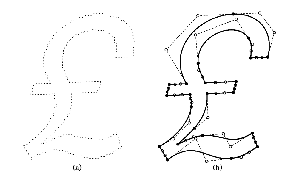
Fig. 75 Figure from the book GraphicGems (1st ed.) where the algorithm was presented; original description: “A digitized glyph, showing the original samples and the fitted curves.”
Judging from the figure above, the cubic Bézier curves can also be parametrized to represent lower order curves, i.e. quadratic Béziers or straight lines.
Implementations of this algorithm have been made available, e.g.:
in C (the original implementation published as part of GraphicGems) in this Github repository
unofficial implementations
in Python in this Github repository
in C++ in this Github repository
in JavaScript in this Github repository
Open question
Is this algorithm really the right one to use? We already have cubic Bézier curves; now, we fit cubic Béziers to them again by sampling points from cubic Béziers?
Open question
Maybe the simplification should be applied more selectively – and not to all input samples?
(4) Minimum resolution
In Carlier et al. (2020), the resulting lines and Bézier curves are divided in multiple subsegments if their length is larger than some distance. In Carlier et al. (2020) this threshold distance \(\Delta = 5\) (i.e. 5 pixels in the 256x256 viewport).
Open question
Why do we want this? Does that not create much more opportunity for “mistuning” a long line made out of two points – by breaking it into more line segments?